Case Studies Evaluation
We next present our experience about using PrivApprox in the following two case studies: (i) New York City (NYC) taxi ride, and (ii) household electricity consumption.
Experimental Setup
Cluster setup. We used a cluster of $44$ nodes connected via a Gigabit Ethernet. Each node contains 2 Intel Xeon quad-core CPUs and 8 GB of RAM running Debian 5.0 with Linux kernel 2.6.26. We deployed two proxies with Apache Kafka, each of which consists of $4$ Kafka broker nodes and $3$ Zookeeper nodes. We used $20$ nodes to deploy Apache Flink as the aggregator. In addition, we employed the remaining $10$ nodes to replay the datasets to generate data streams for evaluating our system.
Datasets. For the first case study, we used the NYC Taxi Ride dataset from the DEBS 2015 Grand Challenge. The dataset consists of the itinerary information of all rides across $10,000$ taxies in New York City in 2013. For the second case study, we used the Household Electricity Consumption dataset. This dataset contains electricity usage (kWh) measured every 30 minutes for one year by smart meters.
Queries. For the NYC taxi ride case-study, we created a query: “What is the distance distribution of taxi trips in New York?”. We defined the query answer with $11$ buckets as follows: [0, 1) mile, [1, 2) miles, [2, 3) miles, [3, 4) miles, [4, 5) miles, [5, 6) miles, [6, 7) miles, [7, 8) miles, [8, 9) miles, [9, 10) miles, and [10, $+\infty$) miles.
For the second case-study, we defined a query to analyze the electricity usage distribution of households over the past 30 minutes. The query answer format is as follows: [0, 0.5] Kwh, (0.5, 1] kWh, (1, 1.5] kWh, (1.5, 2] kWh, (2, 2.5] kWh, and (2.5, 3] kWh.
Evaluation metrics. We evaluated our system using four key metrics: throughput, latency, utility, and privacy level. Throughput is defined as the number of data items processed per second, and latency is defined as the total amount of time required to process a certain dataset. Utility is the accuracy loss defined as $| \frac{estimate - exact}{exact} |$, where $estimate$ and $exact$ are the query results produced by applying PrivApprox and the native computation, respectively. Finally, privacy level is calculated using equation 19 in the technical report.
For all measurements, we report the average over $10$ runs.
Results
Scalability
We measured the scalability of the two main system components: proxies and the aggregator. We first measured the throughput of proxies with various numbers of CPU cores (scale-up) and different numbers of nodes (scale-out). This experiment was conducted on a cluster of $4$ nodes. Figure 1 (a) shows that, as expected, the throughput at proxies scales quite well with the number of CPU cores and nodes. In the NYC Taxi case-study, with $2$ cores, the throughput of each proxy is $512,348$ answers/sec, and with $8$ cores (1 node) the throughput is $1,192,903$ answers/sec; whereas, with a cluster of $4$ nodes each with $8$ cores, the throughput of each proxy reaches $2,539,715$ answers/sec. In the household electricity case-study, the proxies achieve relatively a higher throughput compared because the message size is smaller than in the NYC Taxi case-study.
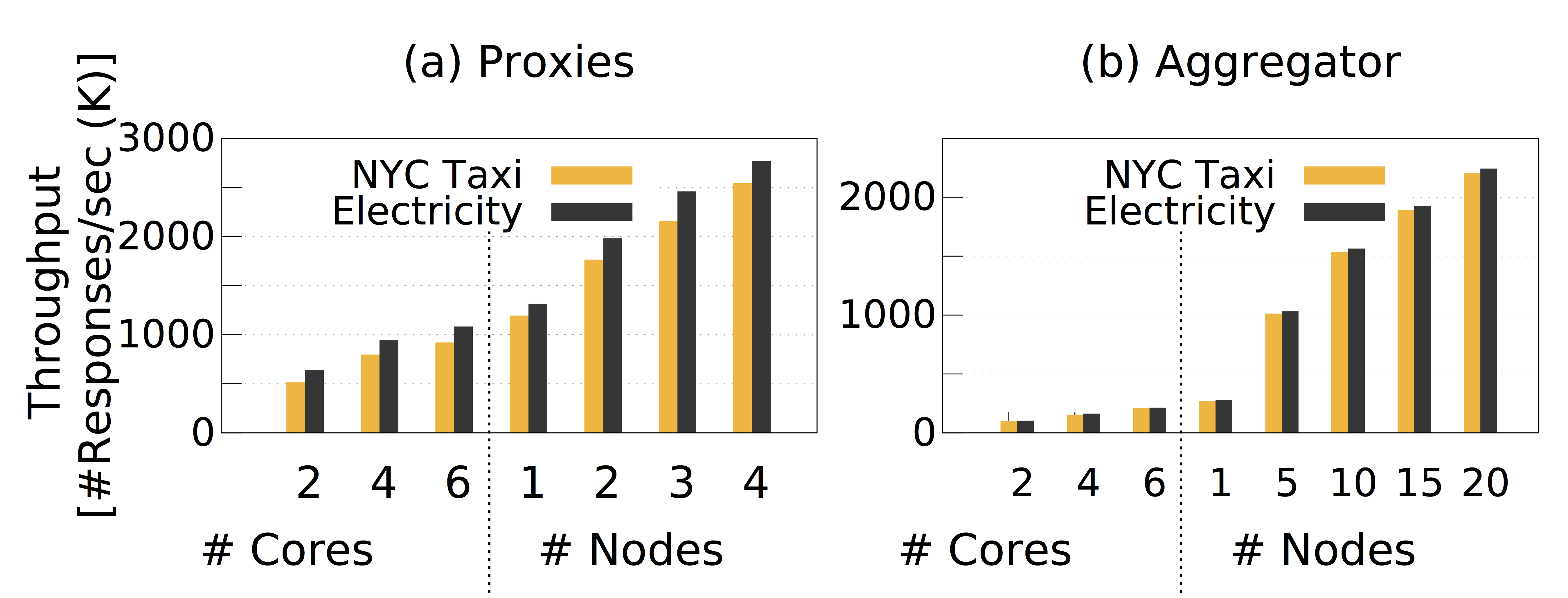
Figure 1: Throughput at proxies and the aggregator with different numbers of CPU cores and nodes.
We next measured the throughput at the aggregator. Figure 1 (b) depicts that the aggregator also scales quite well when the number of nodes for aggregator increases. The throughput of the aggregator, however, is much lower than the throughput of proxies due to the relatively expensive join operation and the analytical computation at the aggregator. We notice that the throughput of the aggregator in the household electricity case study does not significantly improve in comparison to the first case study. This is because the difference in the size of messages between the two case studies does not affect much on the performance of the join operation and the analytical computation.
Network Bandwidth and Latency
Next, we conducted the experiment to measure the network bandwidth usage. By leveraging the sampling mechanism at clients, our system reduces network traffic significantly. Figure 2 (a) shows the total network traffic transferred from clients to proxies with different sampling fractions. In the first case study, with the sampling fraction of $60$%, PrivApprox can reduce the network traffic by $1.62\times$; whereas in the second case study, the reduction is $1.58\times$.
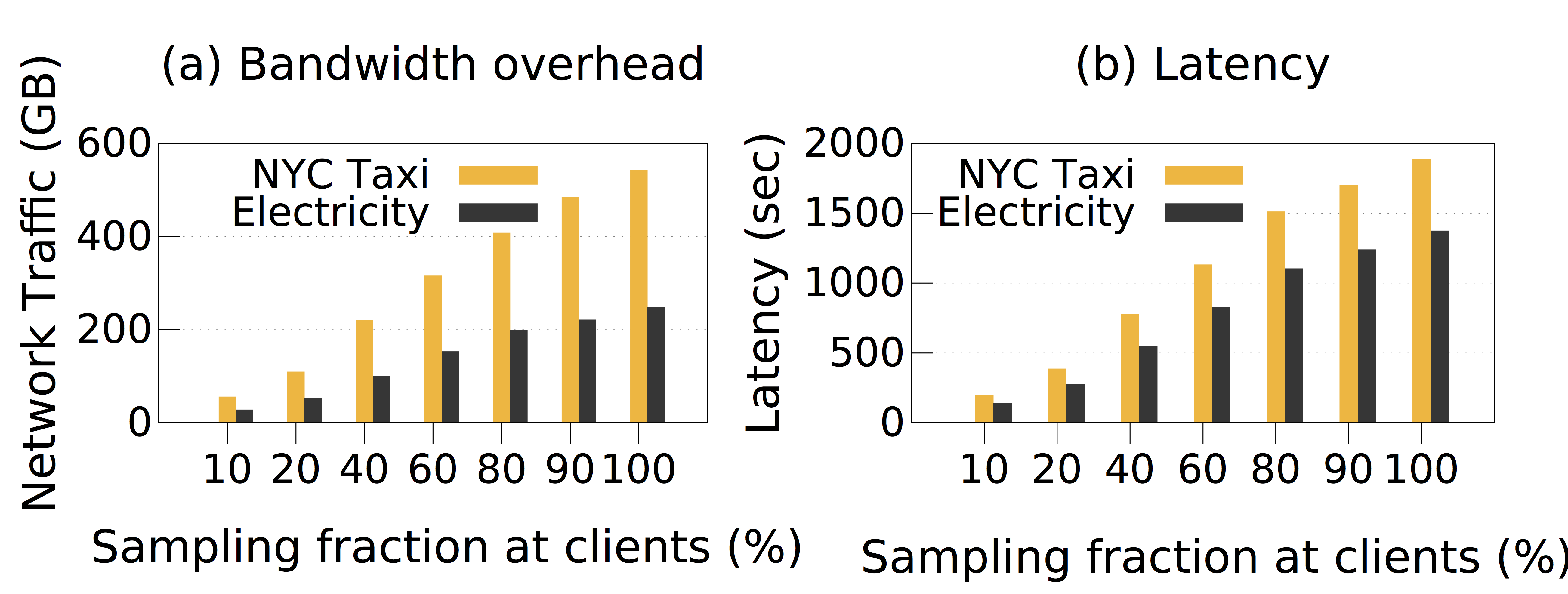
Figure 2: Total network traffic and latency at proxies with different sampling fractions at clients.
Besides the benefit of saving network bandwidth, PrivApprox achieves also lower latency in processing query answers by leveraging approximate computation. To evaluate this advantage, we measured the effect of sampling fractions on the latency of processing query answers. Figure 2 (b) depicts the latency with different sampling fractions at clients. For the first case-study, with the sampling fraction of $60$%, the latency is $1.68\times$ lower than the execution without sampling; whereas, in the second case-study this value is $1.66 \times$ lower than the execution without sampling.
Utility and Privacy
Figure 3 (a)(b)(c) show the utility, the privacy level, and the trade-off between them, respectively, with different sampling and randomization parameters. The randomization parameters $p$ and $q$ are varied in the range of (0, 1), and the sampling parameter $s$ is calculated using equation 19 in the technical report. Here, we show results only for NYC Taxi dataset. As the sampling parameter $s$ and the first randomization parameter $p$ increase, the utility of query results improves (i.e., accuracy loss gets smaller) whereas the privacy guarantee gets weaker (i.e., privacy level gets higher). Since the New York taxi dataset is diverse, the accuracy loss and the privacy level change in a non-linear fashion with different sampling fractions and randomization parameters.
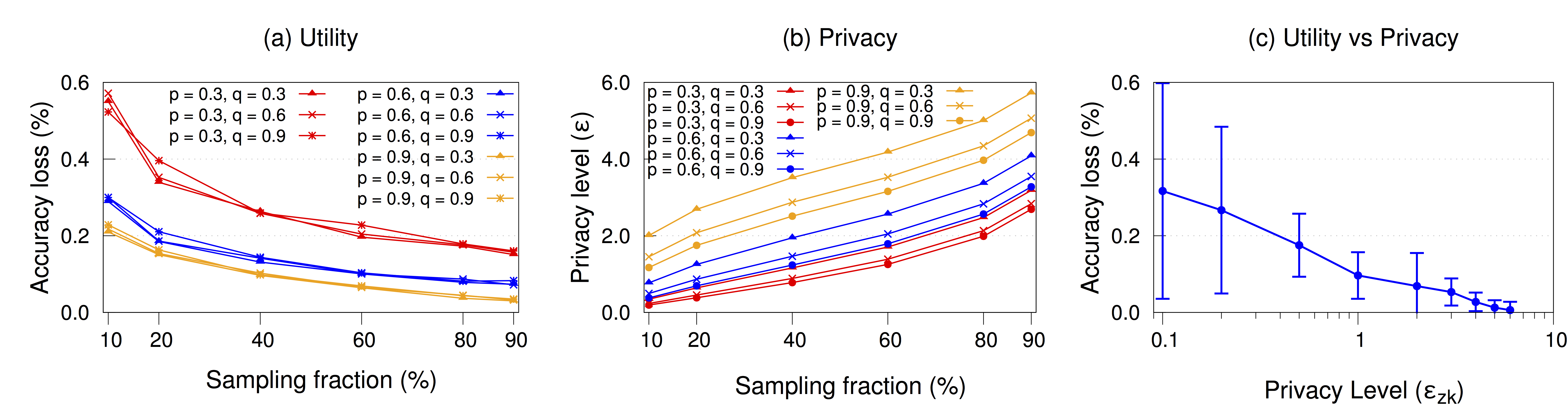
Figure 3: Results from the NYC taxi case-study with varying sampling and randomization parameters: (a) Utility, (b) Privacy level, (c) Comparison between utility and privacy.
Interestingly, the accuracy loss does not always decrease as the second randomization parameter $q$ increases. The accuracy loss gets smaller when $q = 0.3$. This is due to the fact that the fraction of truthful “Yes” answers in the dataset is $33.57$% (close to $q=0.3$).
Historical Analytics
To analyze the performance of PrivApprox for historical analytics, we executed the queries on the datasets stored at the aggregator. Figure 4 (a) (b) present the latency and throughput, respectively, of processing historical datasets with different sampling fractions. We can achieve a speedup of $1.86 \times$ over native execution in historical analytics by setting the sampling fraction to $60$%.
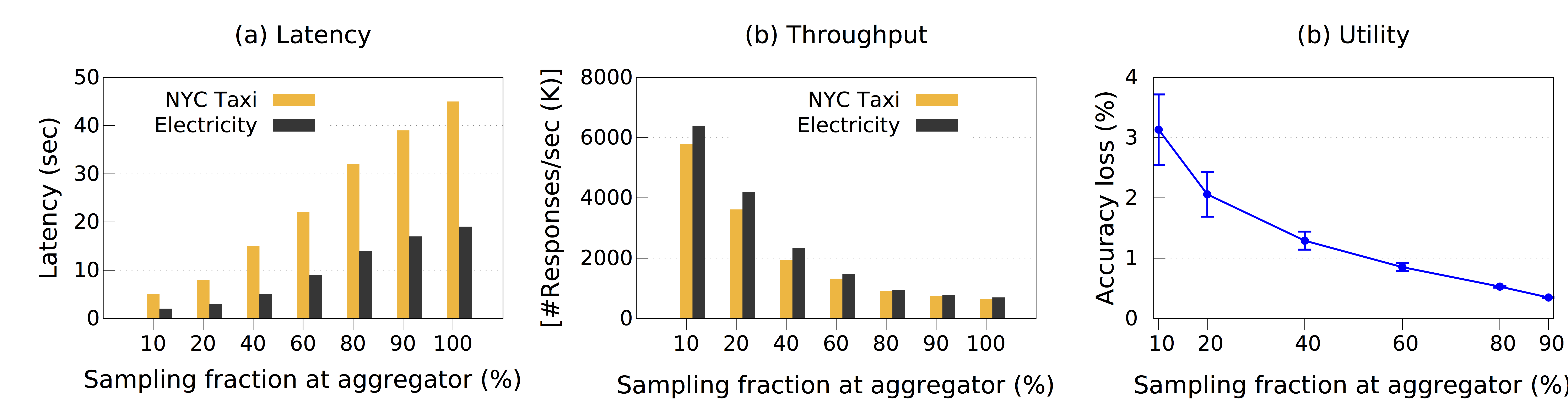
Figure 4: Historical analytics results w/ varying sampling fractions: (a) Latency, (b) Throughput, and (c) Utility.
We also measured the accuracy loss when the approximate computation was applied (for the NYC Taxi case-study). Figure 4 (c) shows the accuracy loss in processing historical with different sampling fractions. With the sampling fraction of $60$%, the accuracy loss is only less than $1$%.